Algorithms in TypeScript
Published: 13/05/25
- Overview
- Measuring Performance
- Option 1: Manually timing it
- Option 2: Spot a trend
- Option 3: Derive Big O via Asymptotic Analysis
- Option 4: Quickly Estimating Time Complexity
- Common algorithms
- Constant Time Complexity
- Logarithmic Time Complexity
- Linear Time Complexity
- Quadratic Time Complexity
- Exponential Time Complexity
- Common Misconception: Calling functions with their own time complexity
- Math Algorithms
- Fibonacci Sequence
- Is Prime
- Min Value in array
- Is Even
- Is Power of Two
- Calculate Factorial
- Recursion
- Calculate Factorial using Recursion
- Fibonacci Sequence using Recursion
- Dynamic Programming
- Fibonacci Sequence using Recursion and Memoisation
- Search Algorithms
- Linear Search
- Binary Search
- Binary Search using Recursion
- The Master Theorem
- Sorting Algorithms
- Bubble Sort
Overview
Algorithms are a sequence of steps to solve a problem. Given the same steps + inputs, an algorithm should always lead to the same solution.
Measuring Performance
Since a problem may have multiple solutions, we often measure the performance of an algorithm to compare.
Option 1: Manually timing it
Note: This approach to measuring algorithm performance is unreliable, more on this below.
Consider the following problem:
Build a function which:
- Takes a number as an input
- Calculates the sum of all numbers leading up to that number
A solution might look like the following:
You might be tempted to measure the performance via the Performance API
Note:
You can change the number in the example below (e.g. to
30), however, don't input large values otherwise your browser will crash (don't go above 300m300000000)Small numbers show
0since the function call finishes in less than a millisecond.
As you make the number bigger, you'll notice that the time it takes increases. However, try the same number twice, it's always slightly different. This is due to various factors:
- The speed of your computer
- The amount of processes running on your computer
- The ram your browser has available
So this isn't the best way to measure the performance of an algorithm.
Option 2: Spot a trend
Note: This approach better than manually timing, however, there's a smarter approach. More on this below.
In the example above, as you add 0's, we see a trend which is roughly:
- 1
- 10
- 100
- 1000
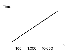
It's a factor of 10 (if we x10 the input, the time it takes is x10 longer). Similarly, if we x2 the input, the time it takes is x2.
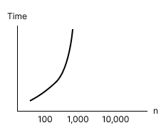
In other words, as the input increases, so does the time in a linear fashion. This trend is called linear time complexity. This is how it would look on a graph:
We could also solve the same problem with a fancy maths formula like so:
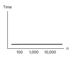
As you add 0's to the example above, you'll notice that the time it takes (looking for a trend, not the exact numbers)
doesn't increase. This trend is called constant time complexity:
These trends are often described using Big O notation (a category for the growth rate of algorithms):
- Linear =
O(n)(pronounced "O of n") - Constant =
O(1)(pronounced "O of 1")
We'll see more later.
Option 3: Derive Big O via Asymptotic Analysis
Note: This approach is the most reliable and wildely used approach to measure an algorithms performance, and we'll be refering to it often in this article.
Asymptotic Analysis is a technique to figure out if an algorithm is Linear O(n), Constant O(1), etc...
It involes 3 steps:
- Define the mathematical "function"
- Find the "fastest growing term" in the mathematical function
- Remove the "coefficient" from the fastest growing term
Let's use Asymptotic Analysis for this function:
function sum(n: number): number {
  let result = 0;

  for (let i = 0; i <= n; i++) {
    result += i;
  }

  return result;
}
Step 1: Define the mathematical function
To figure out the mathematical function, we need to count the number of expression executions.
Let's start off by checking how many times each expression executes when n is 1:
function sum(1: number): number {
  let result = 0; // 1 expression execution

  for (let i = 0; i <= 1; i++) { // 1 expression execution
    result += i; // 1 expression execution
  }

  return result; // 1 expression execution
}
The mathematical "function" is written like so:
T = 1 + 1 + 1 + 1
Where T stands for "Time Complexity".
Now let's check how many times each expression executes when n is 3:
function sum(3: number): number {
  let result = 0; // 1

  for (let i = 0; i <= 3; i++) { // 1
    result += i; // 3
  }

  return result; // 1
}
The mathematical "function" is written like so:
T = 1 + 1 + 3 + 1
So the only thing that changes when n increases is the amount of times the expression in the body of the loop.
Therefore, we can write a generic mathematical function like so:
T = 1 + 1 + n + 1
Which can be shortend to:
T = n + 3
Or
T = 1*n + 3
Note: In the above mathematical function, we've added
1 *beforenwhich may seem redundant in this example, however, explicitly adding1 *will help when dealing with more complex expressions where the values related tonneed to be clearly separated from other constant values
However, we don't need to be this precise. For example, if we always count all expression executions, we would consider a algorithm slower just by adding a line of code e.g:
function sum(n: number): number {
  let result = 0;

  for (let i = 0; i <= n; i++) {
    console.log("...");
    result += i;
  }

  return result;
}
But even with the new line added in the example above, the "big picture" / "trend" / "growth rate" of this algorithm hasn't changed. We're less concerned about exact number of code exections, and more so about the type of mathematical function.
So we can rewrite our mathematical function from:
T = 1*n + 3
to:
T = a*n + b
Which is more generalised. We've replaced the concrete numbers with coefficients (a coefficient is numerical or constant multiplier in an algebraic term):
ais the coefficient of the variablenbis a constant term (not a coefficient of a variable)
Step 2: Find the fastest growing term
For this function:
T = a*n + b
the fastest growing term is a*n, since b is a constant term which doesn't grow
at all, it's always exactly the same number. a*n on the other hand depends
on n, and for a bigger n, this term is bigger.
Step 3: Remove the coefficient from the fastest growing term
For the fastest growing term:
a*n
The coefficient is a in this case, so the mathematical function becomes:
T = n
This tells us that the time complexity for this algorithm depends on n. This is where the n in the
Big O notation for linear time complexity O(n) comes from.
Option 4: Quickly Estimating Time Complexity
As you become comfortable calculating with deriving Big O via Asymptotic Analysis, there are a few ways to quickly spot the time complexity of an algorithm:
- No loop?
- Likely constant
O(1)
- Likely constant
- Loop that repeatedly divides the input number?
- Likely logarithmic
O(log n)
- Likely logarithmic
- Single loop?
- Likely linear
O(n)
- Likely linear
- Nested loop?
- Likely quadratic
O(n²)
- Likely quadratic
- Recursive function that calls itself twice?
- Likely exponential
O(2ⁿ)
- Likely exponential
Let's do another example.
Let's follow the steps to use Asymptotic Analysis to derive Big O for the constant time function discussed earlier:
function sum(n: number): number {
  return (n / 2) * (n + 1);
}
Step 1: define the mathematical function
Starting with n equal to 1:
function sum(1: number): number {
  return (1 / 2) * (1 + 1); // 1
}
So the mathematical function is:
T = 1
And if we try with n equal to 3:
function sum(3: number): number {
  return (3 / 2) * (3 + 1); // 1
}
Which also has a mathematical function of:
T = 1
So regardless of the value of n, we always get T = 1.
We can't make this mathematical function any more general, since
there is no n in this mathematical function.
Step 2: find the fastest growing term
For this mathematical function:
T = 1
There is no fastest growing term since we only have 1 on the right hand side.
Step 3: remove the coefficient from the fastest growing term
And there is no coefficient to remove since there is no n variable, we only have a constant term 1.
so T = 1 is our final mathematical function for this algorithm.
We take the value on the right-hand side of the equals sign and put in in Big O
notation, O(1), which is an example of a constant time algorithm.
Again, if we were to add an extra line of code:
function sum(n: number): number {
  console.log(...);
  return (n / 2) * (n + 1); // 1
}
This doesn't result in:
T = 1 + 1 -> T = 2 -> O(2)
It's still O(1), because we're concerned about the "trend" rather than concrete numbers. In this
case, the time the function takes to execute doesn't depend on n.
Constant time is the best possible outcome for an algorithm in terms of performance, although it isn't always possible.
Common algorithms
Here's a list of the most common algorithms, ordered from fastest to slowest:
Constant Time Complexity
- Big O Notation:
O(1) - Speed: Extremely Fast
nhas no effect on time
Logarithmic Time Complexity
- Big O Notation:
O(log n) - Speed: Very Fast
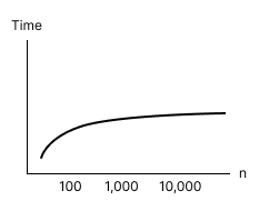
Initially a slow algorithm, but is faster when
nis large because it grows at a slower pace (logarithmically) withn
Linear Time Complexity
- Big O Notation:
O(n) - Speed: Fast
Execution times grows linearly with
n
Quadratic Time Complexity
- Big O Notation:
O(n²) - Speed: Moderate
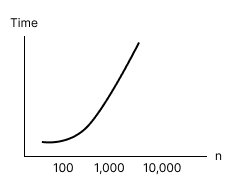
Initially a fast algorithm, but is slower when
nis large because it grows at a faster pace (quadratically) withn
Exponential Time Complexity
- Big O Notation:
O(2ⁿ) - Speed: Extremely Slow.
Execution times grows exponentially with
n
There are even more algorithms (technically any mathematical function is possible), butthese are the most common.
Common Misconception: Calling functions with their own time complexity
Consider this algorithm:
const sumNumbers = (numbers: number[]): number => {
  let result = 0; // 1

  for (const number of numbers) { // 1
    result += number; // n
  }

  return result; // 1
};
Let's follow the steps to use Asymptotic Analysis to derive Big O for this function:
T = 1 + 1 + n + 1T = n + 3T = 1*n + 3T = 1*nT = n
This algorithm has linear time complexity O(n) due to the loop.
We could also impliment this algorithm with a .reduce() like so:
const sumNumbers = (numbers: number[]): number => {
  return numbers.reduce((sum, currNum) => sum + currNum, 0); // under the hood => n
};
But this still has a time complexity of O(n) since .reduce() executes a loop behind the scenes.
Math Algorithms
Fibonacci Sequence
The fibonacci sequence is a series of numbers where each number is the sum of the two preceding numbers:
1, 1, 2, 3, 5, 8, 13, 21, ...
Note: The sequence continues infinitely.
Our task here is:
Write a function that receives an integer and returns the number at that index from the Fibonacci Sequence.
e.g.
fib(4)should return5
Here's the solution:
Let's break it down:
function fib(n: number): number {
  // Create an array to store the fibonacci sequence up to n, starting with the first two numbers
  const numbers = [1, 1];

  // Loop starting at index 2 since we already have those in our array above, and stop when we get
  // to the n + 1 since we want to push the number at index n
  for (let i = 2; i < n + 1; i++) {
    // Sum of the last two numbers in the array above
    numbers.push(numbers[i - 2] + numbers[i - 1]);
  }

  // return the number at index n, which is in the array now
  return numbers[n];
}
This is refereed to as a "bottom-up" approach, meaning westart from an array containing the initial values, and iteratively
build up the Fibonacci sequence from those base cases until we reach the desired value at index n.
Now let's follow the steps to use Asymptotic Analysis to derive Big O for this function:
function fib(n: number): number {
  const numbers = [1, 1]; // 1

  for (let i = 2; i < n + 1; i++) { // 1
    numbers.push(numbers[i - 2] + numbers[i - 1]); // not n, since the loop doesn't start at 0
  }

  return numbers[n]; // 1
}
To see how many times the loop runs, let's add a console log and let dev tools output the count:
When n is 4, the loop runs three times i.e. n - 1 times.
T = 1 + 1 + 1 + n - 1T = n + 2T = 1*n + 2T = 1*nT = n
Therefore this is linear time complexity O(n)
For arguments sake, let's see how the mathematical function would look with an extra expression in the loop
function fib(n: number): number {
  const numbers = [1, 1]; // 1

  for (let i = 2; i < n + 1; i++) { // 1
    console.log("..."); // n - 1
    numbers.push(numbers[i - 2] + numbers[i - 1]); // n - 1
  }

  return numbers[n]; // 1
}
Now let's follow the steps to use Asymptotic Analysis to derive Big O for this function:
T = 1 + 1 + 1 + 2 * (n - 1)T = 3 + 2n - 2T = 2n + 1T = 2nT = n
As you can see, adding another expression execution in the loop still results in T = n, since
the "trend" of this function doesn't change by simply adding an expression in a loop.
Is Prime
The "primality test" determines whether a number is prime (the number can only be divided by itself and 1):
isPrime(9)-> false (divisible by 3)
isPrime(5)-> true
The approach to this problem is to try dividing the input number by all smaller numbers, and return true if it's only divisible by itself and 1.
Here's the solution:
Let's break it down:
function isPrime(num: number): boolean {
  // Loop starting at index 2 since we don't to try dividing by 1, and stop at i < num since
  // we don't want to divide by the number itself
  for (let i = 2; i < num; i++) {
    // If any number divides with no remainder, it's not prime
    if (num % i === 0) {
      return false;
    }
  }

  // Otherwise it is prime
  return true;
}
Now let's follow the steps to use Asymptotic Analysis to derive Big O for this function.
Since we have an if statement, we have different cases with different time complexities, depending on the input number:
- Best case =
O(1)- If
numis1or2, the loop never runs.
- If
- Average case =
O(n)- We don't know the input number; it could be anything between
3and1000003, so a loop is likely to execute.
- We don't know the input number; it could be anything between
- Worst case =
O(n)- If
numis very large and not a prime number (e.g.1000003), the loop finishes without an early return
- If
If an algorithm has different cases, we might have a look at the best and worst cases, but we care most about the average case since we can't predict which case is most likely.
Often the average case has the same time complexity as the worst case scenario due to not knowing which inputs the function will recieve. Usually we calculate the worst case and derive the average case based on that.
However, there's a more efficient solution to this problem due to this mathematical fact:
Every non-prime number (e.g.
9) is produced by two factors (e.g.3and3). At least one of those factors will be smaller or equal to the square root of the number we're analysing.
The square root of a number is a number that when multiplied by itself equals the original number. For 9, the square root is 3.
With this, we can modify our for loop to only loop as many times as Math.sqrt(num) to reduce the amount of loops, and
use <= to check the square root itself:
This changes the Big O of our cases:
- Best case =
O(1) - Average case =
O(sqrt(n)) - Worst case =
O(sqrt(n))
Square root time complexity looks like so on a graph:
More coming soon...
Min Value in Array
Our task here is:
Write a function that receives an array of numbers and returns the minimum value in the array.
e.g.
getMin([1, 2, 3])should return1
Here's the solution:
Pretty self-explanatory.
Now let's follow the steps to use Asymptotic Analysis to derive Big O for this function.
- Best case input:
[1, 2, 3] - Avg case input:
[2, 1, 3] - Worst case input:
[3, 2, 1]
function getMin(numbers: number[]): number {
  let currentMin = numbers[0]; // 1

  for (const num of numbers) { // 1
    if (num < currentMin) { // n
      currentMin = num; // (best) 0; (avg) 1; (worst) 2
    }
  }

  return currentMin; // 1
}
For the worse case:
T = 1 + 1 + n + 2 + 1T = 1*n + 5T = 1*nT = n
All three cases are O(n) since the loop runs in all cases.
Is Even
This one is super simple:
Write a function that receives a number and returns a boolean to determine if the number is even or not.
isEven(1)->false>isEven(2)->true
Here's the solution:
Rather than using Asymptotic Analysis, we can clearly see that there is no loop and there's only one expression execution.
Therefore, this algorithm has a Big O of O(1) i.e. constant time
Is Power of Two
A "power of two" - represented mathematically as 2ⁿ - means the number is produced when you multiply
2 by itself repeatedly (2 x 2 x 2 x ...). The first few powers of 2 are 1, 2, 4, 8, 16, ....
isPowerOfTwo(8)->truevia2³(2 to the power of 3)
isPowerOfTwo(5)->false
The approach to this problem is to continually divide the input number by 2 until we get 1, and as
long as there is no remainder for any division, the number is a power of two.
Here's the solution:
Let's break it down:
function isPowerOfTwo(number: number): boolean {
  // Eliminate 0 and negative numbers
  if (number < 1) {
    return false;
  }

  // A variable to keep track of the current division, started with the input
  let dividedNumber = number;

  // Keep looping until we get to 1
  while (dividedNumber !== 1) {
    // If any division is not divisble by 2, it's not a power of two
    if (dividedNumber % 2 !== 0) {
      return false;
    }

    // Reassign the tracker variable with the next division
    dividedNumber = dividedNumber / 2;
  }

  return true;
}
Now let's follow the steps to use Asymptotic Analysis to derive Big O for this function.
- Best case:
O(1)- With an input of
13, since it's not divisible by 2, the if check in the loop catches it straight away
- With an input of
- Avg case:
O(log n)- Same as below
- Worst case:
O(log n)- With an input of
1,125,899,906,842,624, a very large number which is a power of two (made viaMath.pow(2, 50)) - Large numbers which are a power of two shrink quickly (e.g.
1,000,000is solved in8loops) due to the/ 2 - We don't have
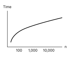
O(n)here since the amount of loops is much smaller thann, we haveO(log n)
- With an input of
A reminder of how O(log n) looks on a graph:
i.e. It doesn't take a large amount of time for big numbers. To prove this, we can count the number of loops via a counter variable:
Calculate Factorial
The factorial of a number is calculated by repeatedly multiplying it by decreasing integers, starting from the number itself, until you reach one. For example:
factorial(3)->3 * 2 * 1=6
The approach to this problem is to iterate through all smaller numbers and multiplying them.
Here's the solution:
Let's break it down:
function factorial(number: number): number {
  // A counter variable for the result, starting at one since `0` would result in 0 * X
  let result = 1;

  // The loop from 2 since 1 is accounted for above, and finish at the number
  for (let i = 2; i <= number; i++) {
    // Multiply the current result by the current iteration in the loop
    result *= i;
  }

  return result;
}
Now let's follow the steps to use quickly estimate time complexity for this function.
Since there's only one loop, this is O(n).
Recursion
Recursion is a technique where a function calls itself to solve a problem.
Calculate Factorial using Recursion
Let's look at an example, revisiting the Calculate Factorial problem we just covered:
Let's break it down:
function factorial(number: number): number {
  // Our "Base Case" – This stops the recursive calls when reached
  if (number === 1) {
    return 1;
  }

  // Recursive Step: Call the function itself with a smaller input
  return number * factorial(number - 1);
}
So when we call factorial(3), the first call looks like this:
function factorial(3: number): number {
  // ...

  return 3 * factorial(2);
}
This triggers the second call:
function factorial(2: number): number {
  // ...

  return 2 * factorial(1);
}
And finally, the third call:
function factorial(1: number): number {
  if (number === 1) {
    return 1;
  }

  // ...
}
We made three recursive calls to factorial(). The process unfolds like this:
factorial(3)returns3 * factorial(2)factorial(2)returns2 * factorial(1)factorial(1)hits the base case and returns1
Substituting these values back up the chain, we get: 3 * (2 * 1) = 6.
Therefore, factorial(3) ultimately returns 6.
Now let's follow the steps to use Asymptotic Analysis to derive Big O for this function.
function factorial(number: number): number {
  if (number === 1) { // 1
    return 1; // 1
  }

  return number * factorial(number - 1); // 1 (however, this triggers the function again)
}
Each individual function call has constant time O(1) since there's no loop, however,
we trigger n function calls, therefore our time complexity is:
T = n * O(1)T = O(n)
Therefore this isn't faster than the non-recursive alternate approach, however, less code is needed in this case.
Sometimes recursion can result in a more efficient algorithm.
Fibonacci Sequence using Recursion
Let's look at an example, revisiting the Fibonacci Sequence problem we previously covered:
The fibonacci sequence is a series of numbers where each number is the sum of the two preceding numbers:
1, 1, 2, 3, 5, 8, 13, 21, ...Write a function that receives an integer and returns the number at that index from the Fibonacci Sequence.
e.g.
fib(4)should return5
Let's break it down:
function fib(n: number): number {
  // Since the fib sequence starts with 1, 1, ... - return 1 in these cases
  if (n === 0 || n === 1) {
    return 1;
  }

  // Recursively call fibonacci function for `n - 1` and `n - 2`
  return fib(n - 1) + fib(n - 2);
}
Let's trace what happens when we call fib(4):
fib(4)fib(3)fib(2)fib(1)-> Returns1fib(0)-> Returns1
fib(1)-> Returns1
fib(2)fib(1)-> Returns1fib(0)-> Returns1
As you can see, there are a lot of function calls (9 to be exact) being made as the recursion progresses. Notably, some function calls, like fib(2)
and its subsequent calls, are repeated multiple times.
Let's see the trend:
fib(4)->9function callsfib(5)->15function calls (6more)fib(6)->25function calls (10more)
Each time we increase n, the function calls increases exponentially and therefore we have exponential time complexity O(2ⁿ).
In summary, this recursive approach to the fibonacci sequence performs worse than the loop approach which has O(n)
But how can we distinguish between:
- Quadratic
O(n²) - Qubic
O(n³) - Exponential
O(2ⁿ)
Let's add a counter:
Comparing the same inputs as if we had Quadratic O(n²) time complexity:
- For an input of 5:
5²=5 * 5=25function calls - For an input of 10:
10²=10 * 10=100function calls - ...
The increase in the number of function calls is slower than what we observed with our recursive algorithm.
Comparing the same inputs as if we had Qubic O(n³) time complexity:
- For an input of 5:
5³=5 * 5 * 5=125function calls - For an input of 10:
10³=10 * 10 * 10=1000function calls - For an input of 20:
20³=20 * 20 * 20=8000function calls - ...
The increase in loops is also slower then what we observed with our recursive algorithm.
This confirms that our recursive algorithm is exponential O(2ⁿ).
Dynamic Programming
Dynamic programming combines Recursion with Memoisation to create more efficient recursive solutions.
Memoization is the technique of storing the results of function calls with specific
inputs (e.g. fib(2) from the Fibonacci sequence). This stored result can then be
reused later without needing to re-compute it, saving computational power and improving performance.
Fibonacci Sequence using Recursion and Memoisation
Let's look at an example, revisiting the Fibonacci Sequence using Recursion problem we previously covered:
Let's break it down:
// The shape of our memo object, which looks like:
// { 0: 1, 1: 1, 2: 2, 3: 3, 4: 5, 5: 8 }
// Where the key is input and the value is the result
interface Memo {
  [key: number]: number;
}

// A global object to store the results from our function calls. This allows us to avoid recomputing values
const memo: Memo = {};

function fib(n: number): number {
  // A variable to store the result, which we can store in the memo and return
  let result;

  // If the memo already contains a value for this input 'n', return it directly (memoisation)
  if (memo[n]) {
    return memo[n];
  }

  // Otherwise, calculate the Fibonacci number recursively
  if (n === 0 || n === 1) {
    result = 1;
  } else {
    result = fib(n - 1) + fib(n - 2);
  }

  // Store the calculated result in the memo for future use
  memo[n] = result;

  return result;
}
This improves the performance of our algorithm by avoiding recalculating previously caclulated function calls. Let's check the performance using the same test cases we used for theFibonacci Sequence using Recursion example:
As you can see, much less function calls due to the results in the memo object. The time complexity here is O(n)
However, we can improve this solution by avoiding the use of a global object to store results across all our initial function calls. This is the problem in question:
const memo = {};

function fib(n) {
  // ...
}

// these two function calls share the same memo
fib(5);
fib(6);
Using a global object introduces potential issues if the input values lead to completely different values. This isn't the case for the fibonacci sequence, but it could be for another problem/algorithm.
Here's a version which creates a new memo for each of the initial function calls:
Let's break it down:
interface Memo {
  [key: number]: number;
}

// The function accepts a memo parameter, which will be an empty object
// that gets populated for each of the initial function calls.
// This ensures that each call has its own independent memoisation space.
function fib(n: number, memo: Memo): number {
  let result;

  if (memo[n]) {
    return memo[n];
  }

  if (n === 0 || n === 1) {
    result = 1;
  } else {
    // Pass the memo that's being populated to the inner function calls
    result = fib(n - 1, memo) + fib(n - 2, memo);
  }

  memo[n] = result;

  return result;
}

// Pass an empty memo object to the initial function calls
console.log(fib(5, {}));
console.log(fib(6, {}));
Search Algorithms
Linear Search
Consider the following array:
[4, 8, 3, 2, 10, -5]If we want to find an element in this array, let's say 10, we could use a linear search algorithm.
The linear search algorithm works as follows:
- Loops through each item in an array
- When it finds the element, it stops and returns the index
It works on ordered and unordered lists.
For example:
However, this wouldn't work for reference data types such as objects as you can see by the undefined in the console:
The reason for this is explained nicely by
Primitive vs Reference Values in JavaScript | ui.dev. In summary,
reference data types, such as objects and arrays, are stored in separate places in memory, so { name: "sammy" } === { name: "sammy" }
results in false. However, when we store it in a variable const person = { name: "sammy" }, then person === person results in
true since both references point to the same place in memory
If we wanted it to work for primative and reference data types, we would could do the following:
Let's break it down:
interface Person {
  name: string;
  age: number;
}

function linearSearch(arr: Person[], element: Person): number | undefined {
  for (let i = 0; i < arr.length; i++) {
    // Check if the provided input is an object which isn't null (since `typeof null` returns "object"),
    // and if the `name` property of the input matches the `name` property of the object in the loop
    if (
      typeof element === "object" &&
      element !== null &&
      element.name === arr[i].name
    ) {
      return i;
    }

    // Otherwise we're not working with objects, so strict equality works
    if (arr[i] === element) {
      return i;
    }
  }
}
However, the drawback here is the object must have a name property for this to work, the algorithm is very specific.
We could make it more flexible via a callback function:
Let's break it down:
interface Person {
  name: string;
  age: number;
}

function linearSearch(
  arr: Person[],
  element: Person,
  comparitorFn: (element: Person, item: Person) => boolean
): number | undefined {
  for (let i = 0; i < arr.length; i++) {
    // Check if the provided input is an object which isn't null, and execute the
    // comparitorFn which implements the matching criteria
    if (
      typeof element === "object" &&
      element !== null &&
      comparitorFn(element, arr[i])
    ) {
      return i;
    }

    if (arr[i] === element) {
      return i;
    }
  }
}

console.log(
  linearSearch(
    [
      { name: "Jane", age: 21 },
      { name: "John", age: 23 },
    ],
    { name: "John", age: 23 },
    // Pass the comparitorFn, which recieves the element we're looking for
    // and the item in the loop, and returns a boolean value indicating whether
    // the element matches.
    (element, item) => element.name === item.name
  )
);
Let's analyise the different cases of inputs/time complexities:
- Best case
- The item we're looking for is the first item in the list e.g.
1in[1, 2, 3] O(1)since only one loop happens
- The item we're looking for is the first item in the list e.g.
- Average case
- The list is in a random order
- Likely
O(n)
- Worst case
- The item we're looking for is the last item in the list e.g.
3in[1, 2, 3] O(n)since it loopsnamount of times
- The item we're looking for is the last item in the list e.g.
Binary Search
Binary search is similar to linear search algorithm, however, it:
- Performs better than
O(n)linear time complexity - The list must be ordered, therefore, you need to sort your list first
Consider the following array:
[-5, 8, 10, 13, 18, 21, 25]The binary search algorithm works as follows:
- Find the median/middle number i.e.
13 - Check if that's the item we're looking for
- If not
- Figure out which half of the list the item must be in (since it's sorted)
- Search that half by finding the medium/middle number
- Check if that's the item we're looking for
- Repeat...
In a nutshell, it repeatedly divides the list in half.
Here it is in action:
Let's break it down:
function binarySearch(sortedArr: number[], element: number): number | undefined {
  // Variables to keep track of the search range (the items to look at in a given loop iteration)
  let startIndex = 0;
  let endIndex = sortedArr.length - 1;

  // Keep looping as long as there is search range, since the following code will half the search range each loop
  while (startIndex <= endIndex) {
    // Calculate the middle index, round down to handle even-length arrays, and add it to the startIndex
    // to ensure we're finding the middle element within the current search range, not just the middle of the original array
    const middleIndex = startIndex + Math.floor((endIndex - startIndex) / 2);

    // If the element we're looking for is the item at the middle index, we found it
    if (element === sortedArr[middleIndex]) {
      return middleIndex;
    }

    // Otherwise, if the middle element is smaller than the target element, the target must be in the right half
    if (sortedArr[middleIndex] < element) {
      startIndex = middleIndex + 1; // Move the start index to search the right half
    } else {
      endIndex = middleIndex - 1;  // Move the end index to search the left half
    }
  }
}
Let's see how many times the loop runs:
Two loop iterations to find an element at index 4.
Let's analyise the different cases of inputs/time complexities:
- Best case
- The item we're looking for is in the middle e.g.
2in[1, 2, 3] O(1)since only one loop happens
- The item we're looking for is in the middle e.g.
- Average case
- We don't know where the
- Likely
O(log n)
- Worst case
- The item we're looking for is the first or last item in the list e.g.
1or5in[1, 2, 3, 4, 5] O(log n)(quicker thanO(n)) since we split the list in half each iteration
- The item we're looking for is the first or last item in the list e.g.
Binary Search using Recursion
We can also impliment the binary search algorithm via recursion:
Let's break it down
function binarySearch(
  sortedArr: number[],
  element: number,
  offset: number
): number | undefined {
  let startIndex = 0;
  let endIndex = sortedArr.length - 1;

  // No while loop needed...

  // No need to add the start index this time since we use slice
  // down below which creates a new array to work with
  const middleIndex = Math.floor((endIndex - startIndex) / 2);

  if (element === sortedArr[middleIndex]) {
    // Add the offset to get the correct index in the
    // original array, not the index in the sliced array
    return middleIndex + offset;
  }

  if (sortedArr[middleIndex] < element) {
    startIndex = middleIndex + 1;
    offset += middleIndex + 1; // Increment offset by the elements we're skipping
  } else {
    endIndex = middleIndex;
  }

  // Recursively call the function
  return binarySearch(
    sortedArr.slice(startIndex, endIndex + 1), // send part of the array
    element,
    offset // send how many elements we've skipped
  );
}

console.log(binarySearch([3, 7, 12, 33, 58, 79], 58, 0)); // Start without an offset
A couple of notes on the time complexity of this algorithm:
- It's faster than
O(n)since we're shrinking the array with each recursive call when callingbinarySearch(sortedArr.slice(...)), we're likely dealing withO(log n) - Calling
slice()costs some performance, however, the genereal trend of the time complexity is not impacted by it
Since we're shrinking the array with each recursive call, this algorithm has the same time complexity as the Loop binary search:
- Best case -
O(1) - Average case -
O(log n) - Worst case -
O(log n)
However, if you want to mathematically derive time complexity via a formula, we can use The Master Theorem.
The Master Theorem
Note: Don’t worry if you don’t get all the math in this section, it's designed to give us a practical way to estimate complexity, not to be a deep mathematical proof
If you want a shortcut to quickly estimate time complexity, check out the steps to use quickly estimate time complexity.
The Master Theorem is a formula for estimating the time complexity of recursive functions. It's particularly useful when you break down a problem
by dividing n into smaller chunks – like we did in the Binary Search using Recursion example above.
Importantly, it doesn’t work well with recursive functions that simply call themselves with n - 1.
The runtime of such recursive functions can often be expressed using this formula: 
This notation shows how the runtime grows as the input size (n) increases. The n term indicates linear scaling, while ‘logba’
shows how efficiently the problem is broken down – often by dividing it into smaller subproblems.
Recursive algorithms fall into one of these three categories:
- Recursive Work Dominates: Most of the work happens in the recursive calls. Big O notation for this case:
- Balanced Workload: The work inside and outside the recursion is roughly equal. Big O notation for this case:
- Non-Recursive Work Dominates: Most of the work happens outside the recursive calls. Big O notation for this case:

Key Terms:
a= Number of subproblems the original problem is divided intob= The factor by which the problem size shrinks in each subproblem (dividing by2meansb = 2)f(n)= The time it takes to do the work outside the recursive calls — i.e. splitting, merging, or any other processing
Let's apply it to the Binary Search using Recursion solution:
function binarySearch(sortedArr: number[], element: number, offset: number ): number | undefined {
  let startIndex = 0;
  let endIndex = sortedArr.length - 1;

  const middleIndex = Math.floor((endIndex - startIndex) / 2);

  if (element === sortedArr[middleIndex]) {
    return middleIndex + offset;
  }

  if (sortedArr[middleIndex] < element) {
    startIndex = middleIndex + 1;
    offset += middleIndex + 1;
  } else {
    endIndex = middleIndex;
  }

  return binarySearch(sortedArr.slice(startIndex, endIndex + 1), element, offset);
}
First, let’s calculate the amount of work done by recursive calls via the Master Theorem:
For this algorithm, the recursive call is this line:
binarySearch(sortedArr.slice(startIndex, endIndex + 1), element, offset)a=1(the number of subproblems / how often the function calls itself)b=2(the sub-problem size i.e. are we splitting the array in halves, thirds etc)
Plugging that in to the formula above ‘O(nlogba)’ we get ‘O(nlog21)’
We can put this the ‘log21’ part into a Logarithm calculator
with 1 in the top box and 2 in the bottom box which results in 0.
This results in ‘O(n0)’ which gives us O(1). So the recursive call in this algorithm:
binarySearch(sortedArr.slice(startIndex, endIndex + 1), element, offset)Has a constant runtime O(1) (not the overall algorithm, just the recursive step).
Next, let's calculate the overall algorithm runtime. We need to check whether the recursive step, which
has a time complexity of O(1), does more/less/equal work to the rest of the function. The rest
of the function looks like so:
// ...

let startIndex = 0;
let endIndex = sortedArr.length - 1;

const middleIndex = Math.floor((endIndex - startIndex) / 2);

if (element === sortedArr[middleIndex]) {
  return middleIndex + offset;
}

if (sortedArr[middleIndex] < element) {
  startIndex = middleIndex + 1;
  offset += middleIndex + 1;
} else {
  endIndex = middleIndex;
}

// ...
Since there isn't a loop or nested function calls (other than Math.floor() which has a time complexity of O(1)),
the rest of the function is O(1). Therefore, since the time complexity of the recursive step O(1) is the same as the
time complexity of the rest of the function O(1), we have this case:
- Same amount of work inside and outside of the recursion
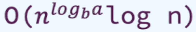
So the overall algorithm time complexity = ‘O(nlogba * log n)’
We calculated the first part ‘nlogba’ earlier via the logarithm calculator which gave us 1, so we have O(1 * log n) which
results in O(log n)
Sorting Algorithms
Bubble Sort
The bubble sort algorithm works by:
- Comparing two items at a time + sort
- Move on to the next two items in the array
- Repeat...
Consider the following array:
[1, 3, -1, 5, 2, 4, 6]If we were using bubble sort to sort this array in ascending order, the algorithm:
- 1st item
- looks at the 1st and 2nd items to begin with
[1, 3, ...]and leaves them as is - looks at the 1st and 3rd
[1, ..., -1]and swaps them[-1, ..., 1] - looks at the 1st and 4th
[-1, ..., ..., 5]and leaves them as is- Notice how, even though the first item was swapped before, we continue to look at the first item in the array
- etc
- looks at the 1st and 2nd items to begin with
- 2nd item
- looks at the 2nd and 3rd
[..., 3, 1, ...]and swaps them[..., 1, 3, ...]- Notice how it no longer looks at the first item
- etc
- looks at the 2nd and 3rd
Here's how it looks in code for ascending order:
For decending order, simply swap > with < in the code editor above.
To be continued...